Profiling and Optimizing a CIFAR10 DDPM Training Loop
I have a simple DDPM UNet training loop in PyTorch on CIFAR-10 that looks like this:
...
running_loss = 0.0
for step in tqdm(range(n_train_steps), total=n_train_steps):
    batch, _ = next(train_loader)

    model.train()
    batch = batch.to("cuda", non_blocking=True)
    with torch.autocast(device_type="cuda", dtype=torch.bfloat16):
        loss = ddpm.forward_batch(batch)
    loss.backward()
    running_loss += loss.item()
    torch.nn.utils.clip_grad_norm_(model.parameters(), max_norm=1.0)
    optimizer.step()
    optimizer.zero_grad(set_to_none=True)
    ema_ddpm.model.update(ddpm.model)
...
The model is similar to the CIFAR-10 UNets proposed in the original DDPM Paper and the Improved DDPM Paper:
- 32M parameters
- Attention at 16x16, 8x8, and 4x4 resolution
- UNet channel sizes of
[128, 256, 256, 256] - 2 residual blocks per stage
The model is trained with batch size 128 with AdamW.
My goal is to improve per-step runtime using only systems-level changes.
Benchmark Setup
All benchmarks are performed on an RTX 4070. To make the benchmarks as consistent as possible, the core and memory clocks were locked to their boost frequencies like so:
nvidia-smi --lock-gpu-clocks=2475
nvidia-smi --lock-memory-clocks=10501
The benchmark times are calculated by performing 5 warmup steps and then timing for 50 steps. We report the mean per-step time and timing is performed around the whole training step so we count: data-loader waiting, data transfer/copy, forward/backward, grad clipping, optimizer, and EMA updates in our runtimes.
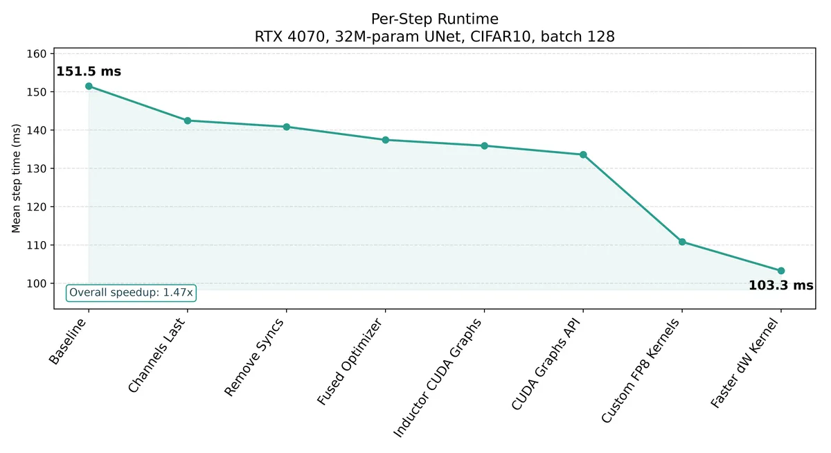
| Optimization | Time (ms) | Speedup (Incremental) | Speedup (Total) |
|---|---|---|---|
| 0. Baseline | 151.48 | - | 1.00x |
| 1. Channels Last | 142.50 | 1.06x | 1.06x |
| 2. Remove Syncs | 140.87 | 1.01x | 1.07x |
| 3. Fused Optimizer | 137.45 | 1.02x | 1.10x |
| 4. Inductor CUDA Graphs | 135.93 | 1.01x | 1.11x |
| 5. CUDA Graphs API | 133.60 | 1.02x | 1.13x |
| 6. Custom FP8 Kernels | 110.82 | 1.21x | 1.37x |
| 7. Faster dW Kernel | 103.28 | 1.07x | 1.47x |
Baseline (151.48ms)
We'll start from a not-totally-sandbagged baseline by applying torch.compile to the model and using bf16 mixed precision. Using this, our per step runtime is 151.48ms. As we are on a GPU with too few SMs, Inductor won't generate optimized GEMM or conv kernels in Triton. The primary benefits from using Inductor are in generating fused non-GEMM kernels.
The two main fusions performed by Inductor are fusing each of these op chains into a single kernel each: F.silu(self.norm1(x)) and self.dropout(F.silu((w + 1) * self.norm2(x) + b)).
Optimization 1 - Channels Last (142.50ms)
Looking at the tensorboard trace, we can see that every conv is sandwiched between two operations: cudnn::engines_precompiled::nchwToNhwcKernel and cudnn::engines_precompiled::nhwcToNchwKernel:
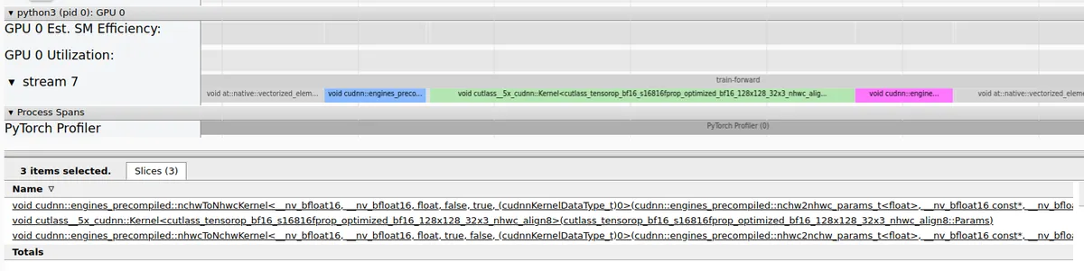
The reason this is done is that a channels-last ordering (nchwToNhwcKernel) makes the convolution's reduction dimension contiguous (Cin for the weight and RxSxCin for the activation) which improves the conv performance at the cost of two extra copies. The profiler shows that approximately 12% of the total train step runtime is taken up by these two kernels. A simple fix here is to perform a global conversion of all the convolution weights one time in the model like so:
...
model = model.to(memory_format=torch.channels_last)
...
We will also need to convert any input we pass into the model to use this channels-last form as well:
batch = batch.to(memory_format = torch.channels_last)
Applying these two modifications gives us a new best time of 142.50ms, a 6 percent speedup, roughly half of what we expected from this optimization.
If we look at the operation chain around convolutions we can see that the previously fully-fused triton_red_fused__to_copy_native_group_norm_silu_6 kernel (which does the GroupNorm + SiLU fusion on an NCHW tensor) is now factored into two separate kernels: triton_red_fused__to_copy_clone_native_group_norm_6 and triton_poi_fused__to_copy_clone_convolution_native_group_norm_silu_7
to support the correct GroupNorm channels-last layout. Computing a channels last GroupNorm is less efficient as all the values required to compute the statistics are no longer contiguous in memory and cannot be loaded as optimally.
Optimization 2 - Reducing CPU <-> GPU Syncs (140.87ms)
Every step we call loss.item() to fetch the current loss value and record it to a CPU tensor. This forces a CPU <-> GPU sync meaning we cannot queue up the grad clip, optimizer update, and ema update kernels asynchronously.
The trace before contains a bubble between when backward ends and grad-clip begins (as well, due to the grad clip kernel being quite quick to execute, we get a secondary bubble for the optimizer step kernel as well):
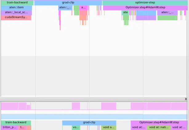
Moving this .item() call to just accumulating into a torch device tensor removes this and we no longer have the bubble:
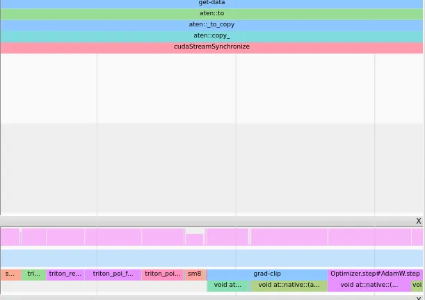
Not a huge speedup, we shave off 2ms and are down to 140.87ms
Optimization 3 - Fused Optimizer (137.45ms)
Just set fused = True for AdamW optimizer. We shave another ~3ms here, runtime is now 137.45ms.
Optimization 4 - Inductor CUDA Graphs (135.93ms)
We previously only compiled the actual UNet forward and backward pass, but a full DDPM training step is more than just that. The ddpm.forward_batch(batch) function we have looks like:
...
def forward_batch(self, batch: torch.Tensor) -> torch.Tensor:
    batch, batch_real, target, t = self.noise_batch(batch)
    eps_pred = self.model(batch, t) # already compiled
    l_simple = F.mse_loss(eps_pred, target)
    return l_simple
...
The noise_batch function itself applies the forward noising process:
x_t = (alpha_bar.sqrt() * x) + ((1.0 - alpha_bar).sqrt() * eps)
which is currently an unfused elementwise operation.
We wrap this whole function with torch.compile(mode = 'reduce-overhead') to allow additional fusion of these operations and the use of CUDA graphs. We lose another 2ms here, the runtime is now 135.93ms.
Optimization 5 - CUDA Graphs API (133.60ms)
There is nothing stopping us from capturing more than just the forward and backward passes in a CUDA graph in this training loop. We can also add the gradient clipping, optimizer step, and EMA update kernels to a graph as well, since these form one atomic training step. I first experimented with creating a train_step function which accomplishes all this and wrapping it with torch.compile(mode = 'reduce-overhead'). This, however, is not ideal as it just creates multiple CUDA Graphs for the forward pass, backward pass, gradient clipping, optimizer step, and EMA update... It could be that I just missed a torch.compile setting but I opted to just use torch's CUDAGraphs API to get the graph I wanted.
With real CUDA graphs implemented, we can see that the host trace is simply doing the data loading and cudaGraphLaunch: 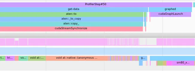
Another 2ms falls here and we are down to 133.60ms.
Optimization 6 - FP8 (110.82ms)
By this stage, I was fairly confident that we were hitting close to optimal performance - GPU utilization is high, we don't see any bubbles in the trace, and there aren't any suspicious looking kernels that take up a large fraction of our runtime. As I am on a GPU that supports FP8 tensor cores an obvious next step would be to switch the training loop over to use FP8, enabling up to a 2x speedup on large GEMMs and convs.
On GPUs with enough SMs, Inductor can actually codegen convs in Triton. The templates for these convs are here which is what I used as my starting point.
For the actual kernels in the UNet, many of them have the following very nice pattern:
- channels in & channels out are powers of 2
- channels last activations and weights
- Most kernels are 3x3, a few are 1x1, all are stride 1
- height / width are also powers of 2
I worked with codex to extract the Triton templates from the above file and simplify the forward and backward kernels given our conditions, which allows us to skip some bounds checks and address calculations.
Click to see the full breakdown of all convolution kernels
| Cin | Cout | in HxW | K | count |
|---|---|---|---|---|
| 256 | 256 | 4x4 | 3x3 | 13 |
| 256 | 256 | 16x16 | 3x3 | 9 |
| 256 | 256 | 8x8 | 3x3 | 9 |
| 128 | 128 | 32x32 | 3x3 | 7 |
| 3 | 128 | 32x32 | 3x3 | 1 |
| 128 | 256 | 32x32 | 3x3 | 1 |
| 256 | 256 | 32x32 | 3x3 | 1 |
| 128 | 256 | 32x32 | 1x1 | 1 |
| 512 | 256 | 4x4 | 3x3 | 1 |
| 512 | 256 | 4x4 | 1x1 | 1 |
| 512 | 256 | 8x8 | 3x3 | 1 |
| 512 | 256 | 8x8 | 1x1 | 1 |
| 512 | 256 | 16x16 | 3x3 | 1 |
| 512 | 256 | 16x16 | 1x1 | 1 |
| 512 | 128 | 32x32 | 3x3 | 1 |
| 512 | 128 | 32x32 | 1x1 | 1 |
| 128 | 3 | 32x32 | 3x3 | 1 |
Swapping all convolutions to FP8 is not a free lunch however. Kernels with sufficiently low arithmetic intensity can end up being slower than their bf16 counterparts as the throughput gains from FP8 don't offset the quantization overhead.
A simple model can determine if a kernel benefits from FP8. We should use it if the time to run in FP8 is less than the time to run in bf16:
The total time for an FP8 operation includes the initial quantization cost plus the computation time. The quantization is memory-bound, while the computation can be modeled with the roofline model.
In contrast, the bf16 time is just the compute time:
Here, is the bytes of the activation tensor being quantized, is the peak memory bandwidth, is the total FLOPs, and is the arithmetic intensity of the operation. This is obviously an approximate model as it assumes we will hit 100% of the peak MemBW/FLOPs for all operations, but it is useful to guide our efforts.
Filtering the above kernel list with this model shows that not all kernels will benefit from FP8.
Click to see the full breakdown of speedup by convolution kernel
| Cin | Cout | in HxW | K | count | expected_fp8_speedup |
|---|---|---|---|---|---|
| 256 | 256 | 4x4 | 3x3 | 13 | 1.55 |
| 256 | 256 | 16x16 | 3x3 | 9 | 1.75 |
| 256 | 256 | 8x8 | 3x3 | 9 | 1.71 |
| 128 | 128 | 32x32 | 3x3 | 7 | 1.53 |
| 3 | 128 | 32x32 | 3x3 | 1 | 1.06 |
| 128 | 256 | 32x32 | 3x3 | 1 | 1.77 |
| 256 | 256 | 32x32 | 3x3 | 1 | 1.77 |
| 128 | 256 | 32x32 | 1x1 | 1 | 0.75 |
| 512 | 256 | 4x4 | 3x3 | 1 | 1.55 |
| 512 | 256 | 4x4 | 1x1 | 1 | 0.83 |
| 512 | 256 | 8x8 | 3x3 | 1 | 1.71 |
| 512 | 256 | 8x8 | 1x1 | 1 | 0.88 |
| 512 | 256 | 16x16 | 3x3 | 1 | 1.75 |
| 512 | 256 | 16x16 | 1x1 | 1 | 0.89 |
| 512 | 128 | 32x32 | 3x3 | 1 | 1.57 |
| 512 | 128 | 32x32 | 1x1 | 1 | 0.56 |
| 128 | 3 | 32x32 | 3x3 | 1 | 1.50 |
The kernels from this list that do not benefit are the 1x1 skip connection convs as their arithmetic intensity is too low to justify the quantization cost. To make the kernel optimization more simple, I also dropped the input and output 3x3 convs as their cumulative speedup is not large and they require masking on either the input or output dimensions.
Of course, just because a specific conv type is used more times than another in the UNet, does not mean that they all hold equal weight in optimization. For example, the most used conv operating on 4x4 images has a minuscule cumulative runtime. At bf16, a single kernel call takes 0.060ms. So the cumulative bf16 runtime for all these 4x4 kernels is 0.7904ms or around the same time as it takes for the single 128 in/cout channels conv on 32x32 images.
Finally, we utilize delayed scaling in the forward and backward pass which saves us an extra half-precision read per tensor. With delayed scaling, the validation loss is half a percent higher than the reference loss but this is an acceptable tradeoff.
Going through a few rounds of iteration here on the forward and backward pass kernels gives us a new runtime of 110.82ms. A full breakdown of all the kernels and their throughputs is given in the Appendix.
Optimization 7 - Faster dW kernel (103.28ms)
A final optimization we apply is for the dW kernel. This kernel effectively computes a dY^T @ A = [Cout, NHW] @ [NHW, RSCin] GEMM. In these cases the reduction dimension NHW is much larger than either the Cout or RSCin dimensions (and Cout and RSCin are usually quite small, leading to poor parallelization when blocking solely over tiles of the output result). While this kernel already used split-k for the reduction, it was still hitting suspiciously low throughput numbers for all tested problem sizes and was on-par with the bf16 dW kernel (hitting ~55 TFLOPs@FP8).
As we are in a channels-last layout, the strides of the LHS operand are (1, Cout) and we are walking along the non-contiguous dimension in blocks. On a systems level, there is nothing wrong with this as whenever we do a row-major @ row-major GEMM, the pattern for the RHS operand is similar (i.e. loading along the non-contiguous dimension). However, Triton did not generate efficient code for this layout:
- Huge amounts of
PRMTinstructions for data movement - Scalar
LDSinstead of vectorizedLDSMloads from shared memory - No async pipelining from global -> shared (
LDS.128instead ofLDGSTS.128)
The solution here (found with the help of deepseek-v4-pro) was to pre-transpose the FP8 dY tensor in a separate kernel. Doing this means that the strides of the LHS operand form a row-major layout. With this layout fix, the dW kernel is now consistently faster than its cudnn bf16 counterpart.
With this fix in place, we reach our final runtime of 103.28ms:
Future Improvements
Progress for this type of work slows down significantly between optimizations. Optimizations 1-5 were implemented over the span of a week while Optimizations 6 and 7 took around two weeks of debugging and profiling. There are a few spots left where we can further optimize the runtimes:
- The linear layers in the QKV attention block have sufficient arithmetic intensity to actually benefit from FP8 computation. Using a similar performance model to the one above shows that FP8 would save at most 3-4% of the forward and backward pass runtime.
- The FP8 implicit GEMM kernels could be further improved with a lower-level DSL. Most of the forward pass kernels hit close to their peak throughput but the backward pass performance is less consistent. All kernels (e2e including quantization overhead) are faster than the bf16 versions but many hit under their theoretical peak. Triton cedes the finer grained control we'd need for this in favor of a faster kernel writing experience. If I were going to take these backward kernels further, I'd look into rewriting them in ThunderKittens or TileLang first.
Code for the final training loop and the benchmark scripts is available here
Appendix - Benchmark Results
Implicit GEMM Forward Pass Benchmarks:
Click to expand
| Shape | TFLOPS/s |
|---|---|
| B128 C128->128 32x32 K3 | 98.1 |
| B128 C128->256 32x32 K3 | 104.4 |
| B128 C256->256 16x16 K3 | 103.8 |
| B128 C512->256 16x16 K3 | 107.1 |
| B128 C256->256 8x8 K3 | 90.1 |
| B128 C512->256 8x8 K3 | 95.7 |
| B128 C512->128 32x32 K3 | 111.3 |
| B128 C256->256 32x32 K3 | 111.0 |
Implicit GEMM Backward Pass Benchmarks:
Click to expand
| Shape | TFLOPS/s |
|---|---|
| dX B128 C128->128 32x32 K3 | 78.8 |
| dW B128 C128->128 32x32 K3 | 74.6 |
| dX B128 C128->256 32x32 K3 | 95.5 |
| dW B128 C128->256 32x32 K3 | 78.2 |
| dX B128 C256->256 16x16 K3 | 91.9 |
| dW B128 C256->256 16x16 K3 | 81.6 |
| dX B128 C512->256 16x16 K3 | 84.0 |
| dW B128 C512->256 16x16 K3 | 89.2 |
| dX B128 C256->256 8x8 K3 | 77.3 |
| dW B128 C256->256 8x8 K3 | 69.8 |
| dX B128 C512->256 8x8 K3 | 84.6 |
| dW B128 C512->256 8x8 K3 | 81.3 |
| dX B128 C512->128 32x32 K3 | 84.6 |
| dW B128 C512->128 32x32 K3 | 91.1 |
| dX B128 C256->256 32x32 K3 | 99.2 |
| dW B128 C256->256 32x32 K3 | 88.2 |